This chapter provides a systematic approach to developing reliable and valid measurement scales. We’ll explore all nine critical steps in the scale development process, with interactive examples and R code to reinforce key concepts.
1 Step 1: Determine Clearly What It Is You Want to Measure
The foundation of any good scale is a clear understanding of what you’re trying to measure. Ambiguity at this stage will cascade through the entire development process.
1.1 Theory as an Aid to Clarity
Theoretical frameworks provide the conceptual foundation for your scale by: - Defining the construct in relation to other variables - Specifying the boundaries of what should and shouldn’t be included - Guiding predictions about how the scale should behave
Moving from broad constructs to specific, measurable components:
Specificity Hierarchy
Broad: “Personality” Intermediate: “Extraversion” Specific: “Comfort in social situations with strangers”
1.3 Being Clear About What to Include in a Measure
Inclusion Criteria Checklist: - Does this aspect directly relate to the theoretical definition? - Can this be reliably observed or reported? - Is this distinct from related but different constructs?
# Interactive exercise: Categorize potential itemspotential_items <-c("I enjoy meeting new people", # Core extraversion"I am physically healthy", # Not extraversion"I feel energized in groups", # Core extraversion "I have many friends", # Outcome of extraversion"I speak loudly in conversations"# Behavioral indicator)# Students can categorize these as: Core, Related, Irrelevant
2 Step 2: Generate an Item Pool
2.1 Choose Items That Reflect the Scale’s Purpose
Items should be directly aligned with your theoretical definition and collectively comprehensive of the construct domain.
# Example item pool generation for Academic Self-Efficacyset.seed(123)# Generate example item poolitem_pool <-data.frame(Item_ID =paste0("ASE_", 1:20),Item_Text =c("I can learn difficult academic material","I am confident in my study abilities", "I can complete challenging assignments","I believe I can succeed in my courses","I can understand complex concepts when I try","I am capable of getting good grades","I can handle academic pressure well","I trust my academic judgment","I can solve difficult problems in my field","I am confident in my test-taking abilities","I can manage my study time effectively","I believe in my academic capabilities","I can overcome academic setbacks","I am sure I can learn skills in my major","I can adapt to different teaching styles","I am confident presenting academic work","I can critically evaluate information","I believe I can meet academic standards","I can persist through difficult coursework","I am confident in my academic decisions" ),Domain =rep(c("Ability Beliefs", "Outcome Expectations", "Persistence", "Judgment"), 5))# Display item pool summaryitem_pool %>%count(Domain) %>% knitr::kable(caption ="Item Pool Distribution by Domain")
Item Pool Distribution by Domain
Domain
n
Ability Beliefs
5
Judgment
5
Outcome Expectations
5
Persistence
5
2.2 Redundancy
Planned redundancy is essential in early stages: - Protects against item loss during validation - Allows selection of best-performing items - Ensures comprehensive domain coverage
# Demonstrate redundancy with correlation matrix# Simulate responses to redundant items measuring same facetn_participants <-200true_score <-rnorm(n_participants, mean =0, sd =1)# Three redundant items with different amounts of erroritem1 <- true_score +rnorm(n_participants, 0, 0.3) # Less erroritem2 <- true_score +rnorm(n_participants, 0, 0.5) # Moderate error item3 <- true_score +rnorm(n_participants, 0, 0.7) # More errorredundant_items <-data.frame(Confidence_1 = item1,Confidence_2 = item2, Confidence_3 = item3)# Show correlationscor_matrix <-cor(redundant_items)print(round(cor_matrix, 2))
Initial item pool should be 3-4 times larger than intended final scale
Final Scale Length
Initial Item Pool
5 items
15-20 items
10 items
30-40 items
20 items
60-80 items
2.4 Beginning the Process of Writing Items
Item Writing Guidelines: 1. Use simple, clear language 2. Avoid double-barreled questions 3. Match reading level to target population 4. Ensure items are answerable by all respondents
2.5 Characteristics of Good and Bad Items
# Examples of good vs. poor itemsitem_examples <-data.frame(Quality =c("Good", "Poor", "Good", "Poor"),Item =c("I feel confident when speaking in public","I feel confident when speaking in public and also when writing reports", # Double-barreled"I enjoy social gatherings","Don't you think that social gatherings are usually enjoyable?"# Leading ),Problem =c("Clear, single concept", "Double-barreled", "Direct statement", "Leading question"))knitr::kable(item_examples, caption ="Examples of Good vs. Poor Item Writing")
Examples of Good vs. Poor Item Writing
Quality
Item
Problem
Good
I feel confident when speaking in public
Clear, single concept
Poor
I feel confident when speaking in public and also when writing reports
Double-barreled
Good
I enjoy social gatherings
Direct statement
Poor
Don’t you think that social gatherings are usually enjoyable?
Leading question
2.6 Positively and Negatively Worded Items
Reverse-Coded Items Caution
While reverse-coded items can control for acquiescence bias, they often: - Create method factors unrelated to the construct - Reduce scale reliability - Confuse respondents - Should be used sparingly and with careful consideration
# Simulate effect of reverse-coded items on factor structurelibrary(lavaan)# Generate data with acquiescence biasset.seed(456)n <-300true_construct <-rnorm(n)acquiescence <-rnorm(n, 0, 0.3)# Forward items influenced by both construct and acquiescenceforward1 <- true_construct + acquiescence +rnorm(n, 0, 0.4)forward2 <- true_construct + acquiescence +rnorm(n, 0, 0.4)# Reverse items: construct effect reversed, but acquiescence still positivereverse1 <--true_construct + acquiescence +rnorm(n, 0, 0.4)reverse2 <--true_construct + acquiescence +rnorm(n, 0, 0.4)mixed_scale <-data.frame(Forward1 = forward1,Forward2 = forward2, Reverse1 = reverse1,Reverse2 = reverse2)# Show how reverse items can create artificial factorsfa_result <-fa(mixed_scale, nfactors =2)print(fa_result$loadings, cutoff =0.3)
Loadings:
         MR1    MR2
Forward1         1.031
Forward2         0.673
Reverse1  0.866
Reverse2  0.957

                 MR1   MR2
SS loadings    1.725 1.523
Proportion Var 0.431 0.381
Cumulative Var 0.431 0.812
3 Step 3: Determine the Format for Measurement
3.1 Thurstone Scaling
Historical approach where items are pre-scaled by judges to represent different levels of the attribute. Rarely used today due to: - Labor-intensive development process - Assumption of equal intervals - Limited flexibility
3.2 Guttman Scaling
Cumulative scaling where items form a hierarchy - endorsing a higher item implies endorsing all lower items.
# Example: Math ability Guttman scaleguttman_items <-data.frame(Level =1:5,Item =c("I can add single-digit numbers","I can multiply two-digit numbers", "I can solve linear equations","I can work with quadratic equations","I can solve calculus problems" ),Expected_Pattern =c("11111", "01111", "00111", "00011", "00001"))knitr::kable(guttman_items, caption ="Guttman Scale Example: Math Ability")
Guttman Scale Example: Math Ability
Level
Item
Expected_Pattern
1
I can add single-digit numbers
11111
2
I can multiply two-digit numbers
01111
3
I can solve linear equations
00111
4
I can work with quadratic equations
00011
5
I can solve calculus problems
00001
3.3 Scales With Equally Weighted Items
Most common approach
- items receive equal weight and are summed or averaged.
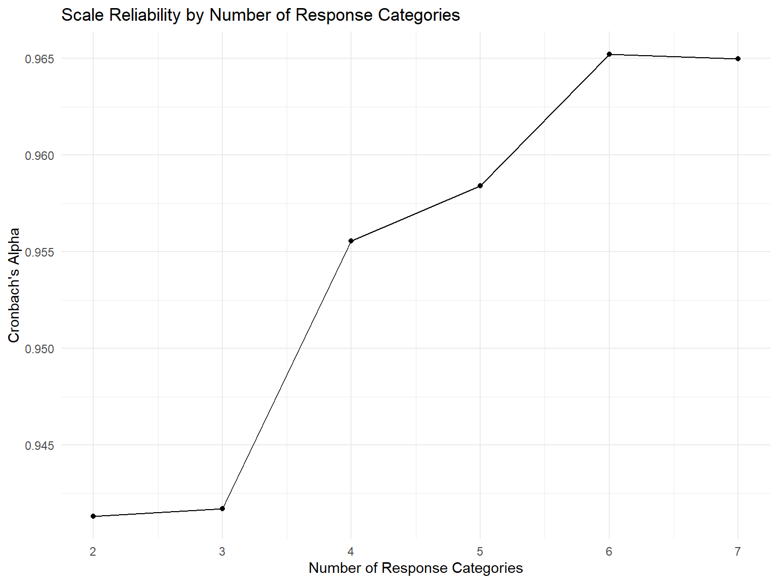
3.4 How Many Response Categories?
# Simulate reliability across different numbers of response optionssimulate_reliability <-function(n_categories, n_items =10, n_people =200) { true_scores <-rnorm(n_people) responses <-matrix(NA, n_people, n_items)for(i in1:n_items) {# Convert continuous to categorical continuous_response <- true_scores +rnorm(n_people, 0, 0.5) responses[,i] <-cut(continuous_response, breaks = n_categories, labels =FALSE) }alpha(responses)$total$raw_alpha}# Test different numbers of categoriescategories <-2:7reliabilities <-sapply(categories, simulate_reliability)reliability_data <-data.frame(Categories = categories,Alpha = reliabilities)# Plot resultsggplot(reliability_data, aes(x = Categories, y = Alpha)) +geom_line() +geom_point() +labs(title ="Scale Reliability by Number of Response Categories",x ="Number of Response Categories",y ="Cronbach's Alpha") +theme_minimal()
3.5 Specific Types of Response Formats
Likert Scale
Most popular format
- statements with agreement levels:
# Example Likert items and response optionslikert_example <-data.frame(Statement =c("I enjoy challenging myself with difficult tasks","I prefer to avoid situations where I might fail","I am motivated by competition with others" ),Response_Options =rep("1=Strongly Disagree, 2=Disagree, 3=Neutral, 4=Agree, 5=Strongly Agree", 3))knitr::kable(likert_example, caption ="Likert Scale Example")
Think-aloud protocols to understand how respondents interpret and process items.
5.1 Cognitive Interview Protocol
Comprehension: “What does this question mean to you?”
Retrieval: “How do you go about answering this?”
Judgment: “How confident are you in your answer?”
Response: “Why did you choose that response option?”
# Common issues identified in cognitive interviewscognitive_issues <-data.frame(Issue_Type =c("Comprehension", "Retrieval", "Judgment", "Response", "Other"),Example =c("Unclear technical terms or jargon","Difficulty recalling relevant experiences", "Uncertain about appropriate reference period","Response options don't match experience","Leading or socially desirable responding" ),Solution =c("Simplify language, add definitions","Provide memory aids or examples","Clarify time frame explicitly", "Expand or modify response options","Reword to reduce bias" ))knitr::kable(cognitive_issues, caption ="Common Cognitive Interview Findings")
Common Cognitive Interview Findings
Issue_Type
Example
Solution
Comprehension
Unclear technical terms or jargon
Simplify language, add definitions
Retrieval
Difficulty recalling relevant experiences
Provide memory aids or examples
Judgment
Uncertain about appropriate reference period
Clarify time frame explicitly
Response
Response options don’t match experience
Expand or modify response options
Other
Leading or socially desirable responding
Reword to reduce bias
5.2 Sample Size for Cognitive Interviews
5-15 participants typically sufficient
Continue until saturation (no new issues emerge)
Include diverse demographic representation
6 Step 6: Consider Inclusion of Validation Items
Strategic inclusion of items to assess convergent and discriminant validity.
6.1 Types of Validation Items
validation_types <-data.frame(Type =c("Convergent", "Discriminant", "Known Groups", "Criterion"),Purpose =c("Should correlate highly with your scale","Should correlate minimally with your scale","Should differentiate between relevant groups", "Should predict important outcomes" ),Example =c("Existing validated scale measuring same construct","Scale measuring theoretically unrelated construct","Expert vs. novice groups on expertise scale","Job performance for job satisfaction scale" ))knitr::kable(validation_types, caption ="Types of Validation Items")
Types of Validation Items
Type
Purpose
Example
Convergent
Should correlate highly with your scale
Existing validated scale measuring same construct
Discriminant
Should correlate minimally with your scale
Scale measuring theoretically unrelated construct
Known Groups
Should differentiate between relevant groups
Expert vs. novice groups on expertise scale
Criterion
Should predict important outcomes
Job performance for job satisfaction scale
6.2 Planning Validation Strategy
# Example validation matrix for Academic Self-Efficacy scalevalidation_matrix <-data.frame(Validation_Scale =c("General Self-Efficacy", "Academic Achievement", "Test Anxiety", "Social Desirability"),Expected_Correlation =c("High Positive (.6-.8)", "Moderate Positive (.3-.5)","Moderate Negative (-.3 to -.5)", "Low (.0-.3)"),Validity_Type =c("Convergent", "Criterion", "Discriminant", "Response Bias"))knitr::kable(validation_matrix, caption ="Validation Strategy for Academic Self-Efficacy")
Validation Strategy for Academic Self-Efficacy
Validation_Scale
Expected_Correlation
Validity_Type
General Self-Efficacy
High Positive (.6-.8)
Convergent
Academic Achievement
Moderate Positive (.3-.5)
Criterion
Test Anxiety
Moderate Negative (-.3 to -.5)
Discriminant
Social Desirability
Low (.0-.3)
Response Bias
7 Step 7: Administer Items to a Development Sample
7.1 Sample Size Considerations
# Sample size guidelines for scale developmentsample_guidelines <-data.frame(Analysis_Type =c("Item Analysis", "Exploratory FA", "Confirmatory FA", "IRT Analysis"),Minimum_N =c("5-10 per item", "5-10 per item", "10-20 per item", "500-1000+"),Recommended_N =c("200+", "300+", "400+", "1000+"),Considerations =c("More stable item statistics","Stable factor structure", "Adequate power for fit indices","Stable item parameters" ))knitr::kable(sample_guidelines, caption ="Sample Size Guidelines by Analysis Type")
Sample Size Guidelines by Analysis Type
Analysis_Type
Minimum_N
Recommended_N
Considerations
Item Analysis
5-10 per item
200+
More stable item statistics
Exploratory FA
5-10 per item
300+
Stable factor structure
Confirmatory FA
10-20 per item
400+
Adequate power for fit indices
IRT Analysis
500-1000+
1000+
Stable item parameters
7.2 Data Collection Best Practices
Data Collection Checklist
✅ Randomize item order (where theoretically appropriate)
✅ Include attention checks to identify careless responding
✅ Balance response options to avoid order effects
✅ Pilot test administration procedures
✅ Plan for missing data handling strategies
# Cronbach's alpha for full scalealpha_full <-alpha(development_df_scored)
Some items ( Item_6 Item_8 Item_10 ) were negatively correlated with the total scale and
probably should be reversed.
To do this, run the function again with the 'check.keys=TRUE' option
# Items that would improve alpha if deletedimprove_alpha <-names(alpha_if_deleted[alpha_if_deleted > alpha_value])if(length(improve_alpha) >0) {cat("\nItems that would improve alpha if deleted:", paste(improve_alpha, collapse =", "))}
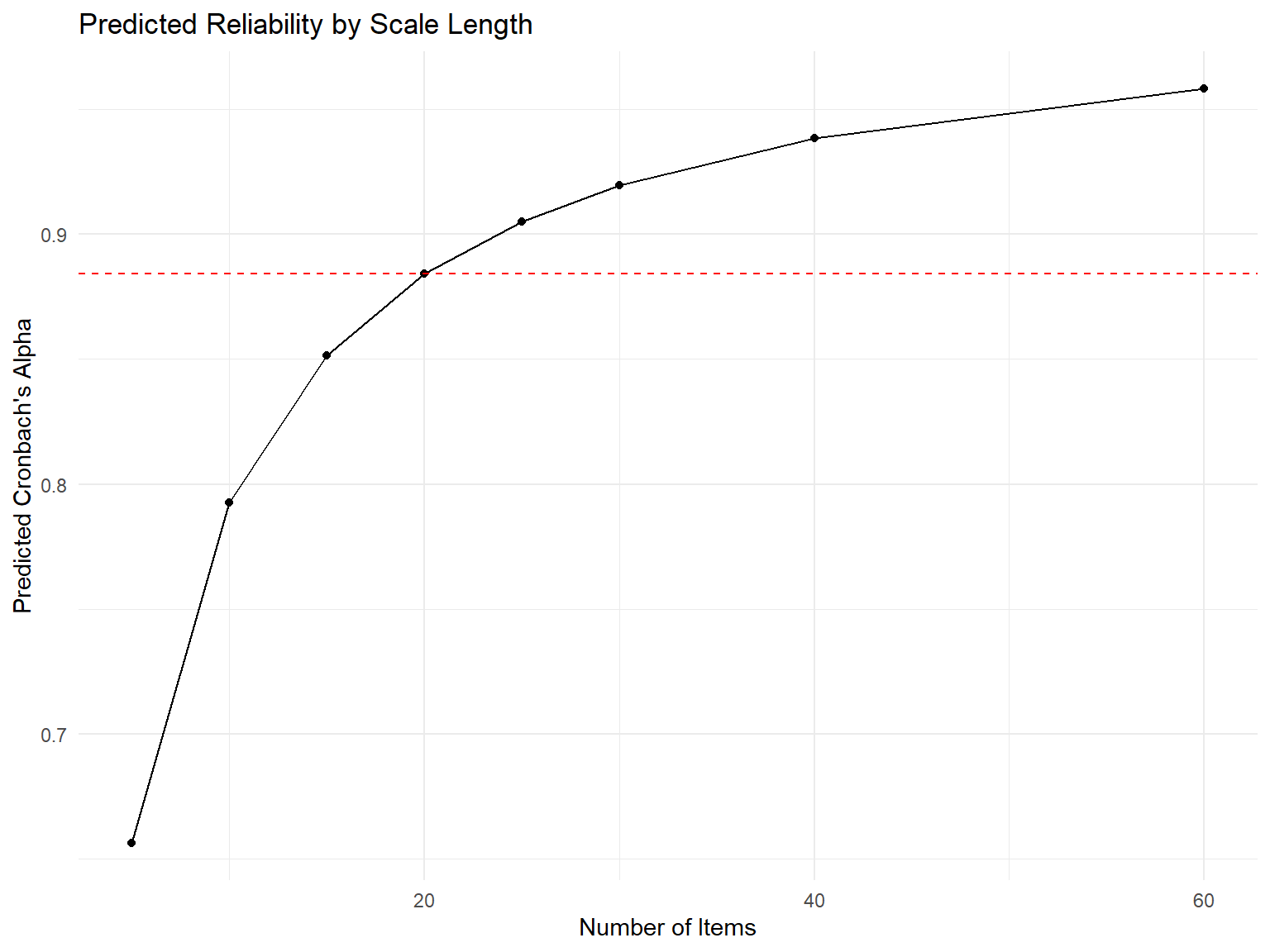
9 Step 9: Optimize Scale Length
9.1 Effect of Scale Length on Reliability
Demonstrate the relationship between scale length and reliability:
# Sequential item removal analysissequential_removal <-function(data, criterion ="alpha") { remaining_items <-names(data) removal_history <-data.frame()while(length(remaining_items) >5) { # Stop at minimum 5 items current_alpha <-alpha(data[remaining_items])$total$raw_alpha# Test removing each item alphas_without <-sapply(remaining_items, function(item) { test_items <-setdiff(remaining_items, item)if(length(test_items) <3) return(NA) # Need minimum itemsalpha(data[test_items])$total$raw_alpha })# Find item whose removal most improves alpha best_removal <-names(which.max(alphas_without)) alpha_improvement <-max(alphas_without, na.rm =TRUE) - current_alphaif(alpha_improvement <=0) break# Stop if no improvement# Record this step removal_history <-rbind(removal_history, data.frame(Step =nrow(removal_history) +1,Removed_Item = best_removal,Items_Remaining =length(remaining_items) -1,Alpha_Before = current_alpha,Alpha_After =max(alphas_without, na.rm =TRUE),Improvement = alpha_improvement ))# Remove the item remaining_items <-setdiff(remaining_items, best_removal) }return(list(history = removal_history, final_items = remaining_items))}# Run sequential removalremoval_results <-sequential_removal(development_df_scored)
Some items ( Item_6 Item_8 Item_10 ) were negatively correlated with the total scale and
probably should be reversed.
To do this, run the function again with the 'check.keys=TRUE' optionSome items ( Item_6 Item_8 Item_10 ) were negatively correlated with the total scale and
probably should be reversed.
To do this, run the function again with the 'check.keys=TRUE' optionSome items ( Item_6 Item_8 Item_10 ) were negatively correlated with the total scale and
probably should be reversed.
To do this, run the function again with the 'check.keys=TRUE' optionSome items ( Item_6 Item_8 Item_10 ) were negatively correlated with the total scale and
probably should be reversed.
To do this, run the function again with the 'check.keys=TRUE' optionSome items ( Item_6 Item_8 Item_10 ) were negatively correlated with the total scale and
probably should be reversed.
To do this, run the function again with the 'check.keys=TRUE' optionSome items ( Item_6 Item_8 Item_10 ) were negatively correlated with the total scale and
probably should be reversed.
To do this, run the function again with the 'check.keys=TRUE' optionSome items ( Item_8 Item_10 ) were negatively correlated with the total scale and
probably should be reversed.
To do this, run the function again with the 'check.keys=TRUE' optionSome items ( Item_6 Item_8 Item_10 ) were negatively correlated with the total scale and
probably should be reversed.
To do this, run the function again with the 'check.keys=TRUE' optionSome items ( Item_6 Item_10 ) were negatively correlated with the total scale and
probably should be reversed.
To do this, run the function again with the 'check.keys=TRUE' optionSome items ( Item_6 Item_8 Item_10 ) were negatively correlated with the total scale and
probably should be reversed.
To do this, run the function again with the 'check.keys=TRUE' optionSome items ( Item_6 Item_8 ) were negatively correlated with the total scale and
probably should be reversed.
To do this, run the function again with the 'check.keys=TRUE' optionSome items ( Item_6 Item_8 Item_10 ) were negatively correlated with the total scale and
probably should be reversed.
To do this, run the function again with the 'check.keys=TRUE' optionSome items ( Item_6 Item_8 Item_10 ) were negatively correlated with the total scale and
probably should be reversed.
To do this, run the function again with the 'check.keys=TRUE' optionSome items ( Item_6 Item_8 Item_10 ) were negatively correlated with the total scale and
probably should be reversed.
To do this, run the function again with the 'check.keys=TRUE' optionSome items ( Item_6 Item_8 Item_10 ) were negatively correlated with the total scale and
probably should be reversed.
To do this, run the function again with the 'check.keys=TRUE' optionSome items ( Item_6 Item_8 Item_10 ) were negatively correlated with the total scale and
probably should be reversed.
To do this, run the function again with the 'check.keys=TRUE' optionSome items ( Item_6 Item_8 Item_10 ) were negatively correlated with the total scale and
probably should be reversed.
To do this, run the function again with the 'check.keys=TRUE' optionSome items ( Item_6 Item_8 Item_10 ) were negatively correlated with the total scale and
probably should be reversed.
To do this, run the function again with the 'check.keys=TRUE' optionSome items ( Item_6 Item_8 Item_10 ) were negatively correlated with the total scale and
probably should be reversed.
To do this, run the function again with the 'check.keys=TRUE' optionSome items ( Item_6 Item_8 Item_10 ) were negatively correlated with the total scale and
probably should be reversed.
To do this, run the function again with the 'check.keys=TRUE' optionSome items ( Item_6 Item_8 Item_10 ) were negatively correlated with the total scale and
probably should be reversed.
To do this, run the function again with the 'check.keys=TRUE' optionSome items ( Item_8 Item_10 ) were negatively correlated with the total scale and
probably should be reversed.
To do this, run the function again with the 'check.keys=TRUE' optionSome items ( Item_8 Item_10 ) were negatively correlated with the total scale and
probably should be reversed.
To do this, run the function again with the 'check.keys=TRUE' optionSome items ( Item_8 Item_10 ) were negatively correlated with the total scale and
probably should be reversed.
To do this, run the function again with the 'check.keys=TRUE' optionSome items ( Item_8 Item_10 ) were negatively correlated with the total scale and
probably should be reversed.
To do this, run the function again with the 'check.keys=TRUE' optionSome items ( Item_8 Item_10 ) were negatively correlated with the total scale and
probably should be reversed.
To do this, run the function again with the 'check.keys=TRUE' optionSome items ( Item_8 Item_10 ) were negatively correlated with the total scale and
probably should be reversed.
To do this, run the function again with the 'check.keys=TRUE' optionSome items ( Item_8 Item_10 ) were negatively correlated with the total scale and
probably should be reversed.
To do this, run the function again with the 'check.keys=TRUE' optionSome items ( Item_10 ) were negatively correlated with the total scale and
probably should be reversed.
To do this, run the function again with the 'check.keys=TRUE' optionSome items ( Item_8 Item_10 ) were negatively correlated with the total scale and
probably should be reversed.
To do this, run the function again with the 'check.keys=TRUE' optionSome items ( Item_8 ) were negatively correlated with the total scale and
probably should be reversed.
To do this, run the function again with the 'check.keys=TRUE' optionSome items ( Item_8 Item_10 ) were negatively correlated with the total scale and
probably should be reversed.
To do this, run the function again with the 'check.keys=TRUE' optionSome items ( Item_8 Item_10 ) were negatively correlated with the total scale and
probably should be reversed.
To do this, run the function again with the 'check.keys=TRUE' optionSome items ( Item_8 Item_10 ) were negatively correlated with the total scale and
probably should be reversed.
To do this, run the function again with the 'check.keys=TRUE' optionSome items ( Item_8 Item_10 ) were negatively correlated with the total scale and
probably should be reversed.
To do this, run the function again with the 'check.keys=TRUE' optionSome items ( Item_8 Item_10 ) were negatively correlated with the total scale and
probably should be reversed.
To do this, run the function again with the 'check.keys=TRUE' optionSome items ( Item_8 Item_10 ) were negatively correlated with the total scale and
probably should be reversed.
To do this, run the function again with the 'check.keys=TRUE' optionSome items ( Item_8 Item_10 ) were negatively correlated with the total scale and
probably should be reversed.
To do this, run the function again with the 'check.keys=TRUE' optionSome items ( Item_8 Item_10 ) were negatively correlated with the total scale and
probably should be reversed.
To do this, run the function again with the 'check.keys=TRUE' optionSome items ( Item_8 Item_10 ) were negatively correlated with the total scale and
probably should be reversed.
To do this, run the function again with the 'check.keys=TRUE' optionSome items ( Item_8 Item_10 ) were negatively correlated with the total scale and
probably should be reversed.
To do this, run the function again with the 'check.keys=TRUE' optionSome items ( Item_10 ) were negatively correlated with the total scale and
probably should be reversed.
To do this, run the function again with the 'check.keys=TRUE' optionSome items ( Item_10 ) were negatively correlated with the total scale and
probably should be reversed.
To do this, run the function again with the 'check.keys=TRUE' optionSome items ( Item_10 ) were negatively correlated with the total scale and
probably should be reversed.
To do this, run the function again with the 'check.keys=TRUE' optionSome items ( Item_10 ) were negatively correlated with the total scale and
probably should be reversed.
To do this, run the function again with the 'check.keys=TRUE' optionSome items ( Item_10 ) were negatively correlated with the total scale and
probably should be reversed.
To do this, run the function again with the 'check.keys=TRUE' optionSome items ( Item_10 ) were negatively correlated with the total scale and
probably should be reversed.
To do this, run the function again with the 'check.keys=TRUE' optionSome items ( Item_10 ) were negatively correlated with the total scale and
probably should be reversed.
To do this, run the function again with the 'check.keys=TRUE' optionSome items ( Item_10 ) were negatively correlated with the total scale and
probably should be reversed.
To do this, run the function again with the 'check.keys=TRUE' optionSome items ( Item_10 ) were negatively correlated with the total scale and
probably should be reversed.
To do this, run the function again with the 'check.keys=TRUE' optionSome items ( Item_10 ) were negatively correlated with the total scale and
probably should be reversed.
To do this, run the function again with the 'check.keys=TRUE' optionSome items ( Item_10 ) were negatively correlated with the total scale and
probably should be reversed.
To do this, run the function again with the 'check.keys=TRUE' optionSome items ( Item_10 ) were negatively correlated with the total scale and
probably should be reversed.
To do this, run the function again with the 'check.keys=TRUE' optionSome items ( Item_10 ) were negatively correlated with the total scale and
probably should be reversed.
To do this, run the function again with the 'check.keys=TRUE' optionSome items ( Item_10 ) were negatively correlated with the total scale and
probably should be reversed.
To do this, run the function again with the 'check.keys=TRUE' optionSome items ( Item_10 ) were negatively correlated with the total scale and
probably should be reversed.
To do this, run the function again with the 'check.keys=TRUE' optionSome items ( Item_10 ) were negatively correlated with the total scale and
probably should be reversed.
To do this, run the function again with the 'check.keys=TRUE' optionSome items ( Item_10 ) were negatively correlated with the total scale and
probably should be reversed.
To do this, run the function again with the 'check.keys=TRUE' optionSome items ( Item_10 ) were negatively correlated with the total scale and
probably should be reversed.
To do this, run the function again with the 'check.keys=TRUE' option
# Split sample for cross-validationset.seed(123)sample_size <-nrow(development_df_scored)split_index <-sample(1:sample_size, size =floor(sample_size *0.5))# Development sample (50%)dev_sample <- development_df_scored[split_index, ]# Validation sample (50%) val_sample <- development_df_scored[-split_index, ]# Develop scale on first halfdev_alpha <-alpha(dev_sample)$total$raw_alpha
Some items ( Item_6 Item_8 Item_10 ) were negatively correlated with the total scale and
probably should be reversed.
To do this, run the function again with the 'check.keys=TRUE' option
dev_item_stats <-describe(dev_sample)# Validate on second halfval_alpha <-alpha(val_sample)$total$raw_alpha
Some items ( Item_6 Item_8 Item_10 ) were negatively correlated with the total scale and
probably should be reversed.
To do this, run the function again with the 'check.keys=TRUE' option
# Test if alphas are significantly differentalpha_difference <-abs(dev_alpha - val_alpha)cat("\nAlpha difference between samples:", round(alpha_difference, 3))
Alpha difference between samples: 0.027
if(alpha_difference <0.05) {cat("\nGood cross-validation: Alpha values are similar")} else {cat("\nCaution: Large difference in alpha between samples")}
Good cross-validation: Alpha values are similar
10 Knowledge Check Exercises
10.1 Exercise 1: Item Quality Assessment
# Evaluate these items - identify problemsexercise_items <-c("I am happy and satisfied with my life","How often do you feel anxious?","I don't not feel uncomfortable in social situations", "My supervisor provides clear guidance and is also fair in evaluations","I am confident in my abilities")# Students should identify: double-barreled, double negative, etc.
10.2 Exercise 2: Response Format Selection
For each construct, recommend the most appropriate response format and justify your choice:
Pain intensity (medical setting)
Brand preference (consumer research)
Frequency of behaviors (behavioral assessment)
Attitude toward policy (political research)
10.3 Exercise 3: Expert Review Analysis
# Given expert ratings, calculate CVR and make decisionsexpert_ratings <-data.frame(Item =paste0("Item_", 1:8),Essential =c(7, 6, 8, 4, 5, 3, 7, 8),Useful =c(1, 2, 0, 3, 2, 4, 1, 0), Unnecessary =c(0, 0, 0, 1, 1, 1, 0, 0))# Calculate CVR for each item (N_experts = 8)# Make retention decisions# Which items need revision?
10.4 Exercise 4: Item Analysis Interpretation
# Interpret these item statistics and make recommendationsmystery_items <-data.frame(Item =c("A", "B", "C", "D", "E"),Mean =c(4.2, 2.1, 3.0, 1.3, 4.8),SD =c(0.6, 1.1, 1.2, 0.5, 0.4),Item_Total_r =c(0.65, 0.72, 0.43, 0.15, 0.28),Alpha_if_deleted =c(0.82, 0.81, 0.83, 0.87, 0.85))# Current alpha = 0.84# Which items would you: Retain, Revise, or Remove?
10.5 Exercise 5: Scale Optimization
Design a strategy for optimizing a 25-item scale where: - Current alpha = 0.78 - 8 items have item-total correlations < 0.30 - Target alpha = 0.85 - Minimum acceptable length = 10 items
10.6 Exercise 6: Item Pool Development
Task: Create a 15-item pool for measuring “Digital Learning Self-Efficacy” - confidence in one’s ability to learn using digital technologies.
✅ Step 1: Construct clearly defined with theoretical foundation
✅ Step 2: Comprehensive item pool generated (3-4x final scale length)
✅ Step 3: Response format selected based on construct and population
✅ Step 4: Expert review completed with content validity assessment
✅ Step 5: Cognitive interviews conducted to refine item wording
✅ Step 6: Validation items strategically included
✅ Step 7: Development sample collected with adequate size
✅ Step 8: Items evaluated through comprehensive psychometric analysis
✅ Step 9: Scale length optimized for reliability and parsimony
Next Steps: Final validation study with independent sample
12 Final Recommendations
Based on the analyses above, here are the key recommendations for your scale:
# Generate final recommendations based on analysesif(exists("removal_results") &&nrow(removal_results$history) >0) { final_items <- removal_results$final_items final_alpha <-alpha(development_df_scored[final_items])$total$raw_alphacat("FINAL SCALE RECOMMENDATIONS:\n")cat("==========================\n")cat("Recommended items:", length(final_items), "\n")cat("Expected reliability:", round(final_alpha, 3), "\n")cat("Items to retain:", paste(final_items, collapse =", "), "\n") removed_items <-setdiff(names(development_df_scored), final_items)if(length(removed_items) >0) {cat("Items to remove:", paste(removed_items, collapse =", "), "\n") }} else {cat("All items performed adequately. Consider minor refinements based on expert feedback.")}
# Generate practice dataset for students to work withset.seed(789)practice_responses <-matrix(sample(1:5, 500, replace =TRUE, prob =c(0.1, 0.2, 0.4, 0.2, 0.1)), nrow =100, ncol =5)colnames(practice_responses) <-paste0("Practice_Item_", 1:5)# Save for later exerciseswrite.csv(practice_responses, "practice_scale_data.csv", row.names =FALSE)# Basic descriptive statisticsdescribe(practice_responses)
14 Key Takeaways
Critical Success Factors
Theoretical Foundation: Always start with clear construct definition
Iterative Process: Scale development requires multiple rounds of refinement
Sample Size: Invest in adequate sample sizes for stable results
Multiple Indicators: Use various psychometric indices, not just Cronbach’s alpha
Cross-Validation: Always validate findings in independent samples
Practical Considerations: Balance psychometric quality with usability
15 Further Reading
For deeper understanding of scale development principles:
DeVellis & Thorpe (2021): Comprehensive guide to all aspects of scale development
Nunnally & Bernstein (1994): Classic text on psychometric theory
Fabrigar et al. (1999): Guidelines for factor analysis in scale development
Sijtsma (2009): Critical perspective on reliability assessment
DeVellis, R. F., & Thorpe, C. T. (2021). Scale development: Theory and applications (5th ed.). SAGE Publications.
Nunnally, J. C., & Bernstein, I. H. (1994). Psychometric theory (3rd ed.). McGraw-Hill.
Fabrigar, L. R., Wegener, D. T., MacCallum, R. C., & Strahan, E. J. (1999). Evaluating the use of exploratory factor analysis in psychological research. Psychological Methods, 4(3), 272–299.
Sijtsma, K. (2009). On the use, the misuse, and the very limited usefulness of cronbach’s alpha. Psychometrika, 74(1), 107–120.
This completes the comprehensive guide to all nine steps of scale development as outlined by DeVellis & Thorpe (2021). The notebook provides both theoretical understanding and hands-on practice with real R code examples.
Source Code
---title: "5. Guidelines in Scale Development"---This chapter provides a systematic approach to developing reliable and valid measurement scales. We'll explore all nine critical steps in the scale development process, with interactive examples and R code to reinforce key concepts.---## Step 1: Determine Clearly What It Is You Want to MeasureThe foundation of any good scale is a clear understanding of what you're trying to measure. Ambiguity at this stage will cascade through the entire development process.### Theory as an Aid to ClarityTheoretical frameworks provide the conceptual foundation for your scale by:- Defining the construct in relation to other variables- Specifying the boundaries of what should and shouldn't be included- Guiding predictions about how the scale should behave```{r theory-framework}# Example: Job Satisfaction construct mappinglibrary(tidyverse)library(psych)library(ggplot2)# Theoretical components of job satisfactionjob_sat_theory <-data.frame(Component =c("Work Content", "Supervision", "Pay", "Colleagues", "Promotion"),Definition =c("Tasks and responsibilities", "Quality of management", "Compensation adequacy", "Peer relationships", "Growth opportunities"),Related_Constructs =c("Job Characteristics", "Leadership", "Equity Theory", "Social Support", "Career Development"))knitr::kable(job_sat_theory, caption ="Theoretical Framework for Job Satisfaction Scale")```### Specificity as an Aid to ClarityMoving from broad constructs to specific, measurable components:::: {.callout-tip}## Specificity Hierarchy**Broad**: "Personality" **Intermediate**: "Extraversion" **Specific**: "Comfort in social situations with strangers":::### Being Clear About What to Include in a Measure**Inclusion Criteria Checklist:**- Does this aspect directly relate to the theoretical definition?- Can this be reliably observed or reported?- Is this distinct from related but different constructs?```{r inclusion-criteria}# Interactive exercise: Categorize potential itemspotential_items <-c("I enjoy meeting new people", # Core extraversion"I am physically healthy", # Not extraversion"I feel energized in groups", # Core extraversion "I have many friends", # Outcome of extraversion"I speak loudly in conversations"# Behavioral indicator)# Students can categorize these as: Core, Related, Irrelevant```---## Step 2: Generate an Item Pool### Choose Items That Reflect the Scale's PurposeItems should be **directly aligned** with your theoretical definition and **collectively comprehensive** of the construct domain.```{r initial-item-pool}# Example item pool generation for Academic Self-Efficacyset.seed(123)# Generate example item poolitem_pool <-data.frame(Item_ID =paste0("ASE_", 1:20),Item_Text =c("I can learn difficult academic material","I am confident in my study abilities", "I can complete challenging assignments","I believe I can succeed in my courses","I can understand complex concepts when I try","I am capable of getting good grades","I can handle academic pressure well","I trust my academic judgment","I can solve difficult problems in my field","I am confident in my test-taking abilities","I can manage my study time effectively","I believe in my academic capabilities","I can overcome academic setbacks","I am sure I can learn skills in my major","I can adapt to different teaching styles","I am confident presenting academic work","I can critically evaluate information","I believe I can meet academic standards","I can persist through difficult coursework","I am confident in my academic decisions" ),Domain =rep(c("Ability Beliefs", "Outcome Expectations", "Persistence", "Judgment"), 5))# Display item pool summaryitem_pool %>%count(Domain) %>% knitr::kable(caption ="Item Pool Distribution by Domain")```### Redundancy**Planned redundancy** is essential in early stages:- Protects against item loss during validation- Allows selection of best-performing items- Ensures comprehensive domain coverage```{r redundancy-example}# Demonstrate redundancy with correlation matrix# Simulate responses to redundant items measuring same facetn_participants <-200true_score <-rnorm(n_participants, mean =0, sd =1)# Three redundant items with different amounts of erroritem1 <- true_score +rnorm(n_participants, 0, 0.3) # Less erroritem2 <- true_score +rnorm(n_participants, 0, 0.5) # Moderate error item3 <- true_score +rnorm(n_participants, 0, 0.7) # More errorredundant_items <-data.frame(Confidence_1 = item1,Confidence_2 = item2, Confidence_3 = item3)# Show correlationscor_matrix <-cor(redundant_items)print(round(cor_matrix, 2))```### Number of Items**Initial item pool should be 3-4 times larger than intended final scale**| Final Scale Length | Initial Item Pool ||-------------------|-------------------|| 5 items | 15-20 items || 10 items | 30-40 items || 20 items | 60-80 items |### Beginning the Process of Writing Items**Item Writing Guidelines:**1. Use simple, clear language2. Avoid double-barreled questions3. Match reading level to target population4. Ensure items are answerable by all respondents### Characteristics of Good and Bad Items```{r item-examples}# Examples of good vs. poor itemsitem_examples <-data.frame(Quality =c("Good", "Poor", "Good", "Poor"),Item =c("I feel confident when speaking in public","I feel confident when speaking in public and also when writing reports", # Double-barreled"I enjoy social gatherings","Don't you think that social gatherings are usually enjoyable?"# Leading ),Problem =c("Clear, single concept", "Double-barreled", "Direct statement", "Leading question"))knitr::kable(item_examples, caption ="Examples of Good vs. Poor Item Writing")```### Positively and Negatively Worded Items::: {.callout-warning}## Reverse-Coded Items CautionWhile reverse-coded items can control for acquiescence bias, they often:- Create method factors unrelated to the construct- Reduce scale reliability- Confuse respondents- Should be used sparingly and with careful consideration:::```{r reverse-coding-demo}# Simulate effect of reverse-coded items on factor structurelibrary(lavaan)# Generate data with acquiescence biasset.seed(456)n <-300true_construct <-rnorm(n)acquiescence <-rnorm(n, 0, 0.3)# Forward items influenced by both construct and acquiescenceforward1 <- true_construct + acquiescence +rnorm(n, 0, 0.4)forward2 <- true_construct + acquiescence +rnorm(n, 0, 0.4)# Reverse items: construct effect reversed, but acquiescence still positivereverse1 <--true_construct + acquiescence +rnorm(n, 0, 0.4)reverse2 <--true_construct + acquiescence +rnorm(n, 0, 0.4)mixed_scale <-data.frame(Forward1 = forward1,Forward2 = forward2, Reverse1 = reverse1,Reverse2 = reverse2)# Show how reverse items can create artificial factorsfa_result <-fa(mixed_scale, nfactors =2)print(fa_result$loadings, cutoff =0.3)```---## Step 3: Determine the Format for Measurement### Thurstone Scaling**Historical approach** where items are pre-scaled by judges to represent different levels of the attribute. Rarely used today due to:- Labor-intensive development process- Assumption of equal intervals- Limited flexibility### Guttman Scaling**Cumulative scaling** where items form a hierarchy - endorsing a higher item implies endorsing all lower items.```{r guttman-scaling}# Example: Math ability Guttman scaleguttman_items <-data.frame(Level =1:5,Item =c("I can add single-digit numbers","I can multiply two-digit numbers", "I can solve linear equations","I can work with quadratic equations","I can solve calculus problems" ),Expected_Pattern =c("11111", "01111", "00111", "00011", "00001"))knitr::kable(guttman_items, caption ="Guttman Scale Example: Math Ability")```### Scales With Equally Weighted Items**Most common approach** - items receive equal weight and are summed or averaged.### How Many Response Categories?```{r response-categories}# Simulate reliability across different numbers of response optionssimulate_reliability <-function(n_categories, n_items =10, n_people =200) { true_scores <-rnorm(n_people) responses <-matrix(NA, n_people, n_items)for(i in1:n_items) {# Convert continuous to categorical continuous_response <- true_scores +rnorm(n_people, 0, 0.5) responses[,i] <-cut(continuous_response, breaks = n_categories, labels =FALSE) }alpha(responses)$total$raw_alpha}# Test different numbers of categoriescategories <-2:7reliabilities <-sapply(categories, simulate_reliability)reliability_data <-data.frame(Categories = categories,Alpha = reliabilities)# Plot resultsggplot(reliability_data, aes(x = Categories, y = Alpha)) +geom_line() +geom_point() +labs(title ="Scale Reliability by Number of Response Categories",x ="Number of Response Categories",y ="Cronbach's Alpha") +theme_minimal()```### Specific Types of Response Formats#### Likert Scale**Most popular format** - statements with agreement levels:```{r likert-format}# Example Likert items and response optionslikert_example <-data.frame(Statement =c("I enjoy challenging myself with difficult tasks","I prefer to avoid situations where I might fail","I am motivated by competition with others" ),Response_Options =rep("1=Strongly Disagree, 2=Disagree, 3=Neutral, 4=Agree, 5=Strongly Agree", 3))knitr::kable(likert_example, caption ="Likert Scale Example")```#### Semantic Differential**Bipolar adjectives** with rating scales between them:```Friendly ___:___:___:___:___:___:___ Unfriendly 1 2 3 4 5 6 7Fast ___:___:___:___:___:___:___ Slow 1 2 3 4 5 6 7```#### Visual Analog**Continuous line** where respondents mark their position:```Not at all confident |________________| Extremely confident 0 100```---## Step 4: Have Initial Item Pool Reviewed by ExpertsExpert review is crucial for establishing **content validity** and identifying potential problems before data collection.### Expert Selection Criteria- Subject matter expertise in the construct domain- Experience with scale development or psychometrics- Representation of key stakeholder perspectives- Typically 3-10 experts depending on construct complexity```{r expert-review}# Expert review evaluation frameworkexpert_criteria <-data.frame(Criterion =c("Relevance", "Clarity", "Comprehensiveness", "Redundancy", "Bias"),Description =c("Does item measure the intended construct?","Is the item clearly worded and unambiguous?", "Do items cover all aspects of the construct?","Are there unnecessary duplicate items?","Are items free from cultural/demographic bias?" ),Rating_Scale =rep("1-4 scale: 1=Poor, 2=Fair, 3=Good, 4=Excellent", 5))knitr::kable(expert_criteria, caption ="Expert Review Evaluation Framework")```### Content Validity Ratio (CVR)Quantify expert agreement on item necessity:```{r cvr-calculation}# Calculate Content Validity Ratiocalculate_cvr <-function(n_essential, n_experts) { cvr <- (n_essential - (n_experts/2)) / (n_experts/2)return(cvr)}# Example: 8 experts, varying levels of agreementexpert_data <-data.frame(Item =paste0("Item_", 1:6),N_Essential =c(8, 7, 6, 5, 4, 2),N_Experts =rep(8, 6))expert_data$CVR <-calculate_cvr(expert_data$N_Essential, expert_data$N_Experts)expert_data$Decision <-ifelse(expert_data$CVR >=0.75, "Retain", ifelse(expert_data$CVR >=0.5, "Revise", "Remove"))knitr::kable(expert_data, caption ="Content Validity Ratio Results", digits =2)```---## Step 5: Cognitive Interviewing**Think-aloud protocols** to understand how respondents interpret and process items.### Cognitive Interview Protocol1. **Comprehension**: "What does this question mean to you?"2. **Retrieval**: "How do you go about answering this?"3. **Judgment**: "How confident are you in your answer?"4. **Response**: "Why did you choose that response option?"```{r cognitive-issues}# Common issues identified in cognitive interviewscognitive_issues <-data.frame(Issue_Type =c("Comprehension", "Retrieval", "Judgment", "Response", "Other"),Example =c("Unclear technical terms or jargon","Difficulty recalling relevant experiences", "Uncertain about appropriate reference period","Response options don't match experience","Leading or socially desirable responding" ),Solution =c("Simplify language, add definitions","Provide memory aids or examples","Clarify time frame explicitly", "Expand or modify response options","Reword to reduce bias" ))knitr::kable(cognitive_issues, caption ="Common Cognitive Interview Findings")```### Sample Size for Cognitive Interviews- **5-15 participants** typically sufficient- Continue until **saturation** (no new issues emerge)- Include diverse demographic representation---## Step 6: Consider Inclusion of Validation ItemsStrategic inclusion of items to assess **convergent** and **discriminant** validity.### Types of Validation Items```{r validation-types}validation_types <-data.frame(Type =c("Convergent", "Discriminant", "Known Groups", "Criterion"),Purpose =c("Should correlate highly with your scale","Should correlate minimally with your scale","Should differentiate between relevant groups", "Should predict important outcomes" ),Example =c("Existing validated scale measuring same construct","Scale measuring theoretically unrelated construct","Expert vs. novice groups on expertise scale","Job performance for job satisfaction scale" ))knitr::kable(validation_types, caption ="Types of Validation Items")```### Planning Validation Strategy```{r validation-strategy}# Example validation matrix for Academic Self-Efficacy scalevalidation_matrix <-data.frame(Validation_Scale =c("General Self-Efficacy", "Academic Achievement", "Test Anxiety", "Social Desirability"),Expected_Correlation =c("High Positive (.6-.8)", "Moderate Positive (.3-.5)","Moderate Negative (-.3 to -.5)", "Low (.0-.3)"),Validity_Type =c("Convergent", "Criterion", "Discriminant", "Response Bias"))knitr::kable(validation_matrix, caption ="Validation Strategy for Academic Self-Efficacy")```---## Step 7: Administer Items to a Development Sample### Sample Size Considerations```{r sample-size}# Sample size guidelines for scale developmentsample_guidelines <-data.frame(Analysis_Type =c("Item Analysis", "Exploratory FA", "Confirmatory FA", "IRT Analysis"),Minimum_N =c("5-10 per item", "5-10 per item", "10-20 per item", "500-1000+"),Recommended_N =c("200+", "300+", "400+", "1000+"),Considerations =c("More stable item statistics","Stable factor structure", "Adequate power for fit indices","Stable item parameters" ))knitr::kable(sample_guidelines, caption ="Sample Size Guidelines by Analysis Type")```### Data Collection Best Practices::: {.callout-tip}## Data Collection Checklist✅ **Randomize item order** (where theoretically appropriate) ✅ **Include attention checks** to identify careless responding ✅ **Balance response options** to avoid order effects ✅ **Pilot test** administration procedures ✅ **Plan for missing data** handling strategies :::```{r simulate-data}# Simulate development sample dataset.seed(2024)n_participants <-300n_items <-20# Simulate true factor structurefactor1 <-rnorm(n_participants, 0, 1) # Primary factorfactor2 <-rnorm(n_participants, 0, 0.3) # Minor method factor# Create item responses with varying qualityitem_loadings <-c(0.8, 0.7, 0.6, 0.75, 0.65, # Good items0.4, 0.45, 0.35, # Marginal items 0.2, 0.15, # Poor items0.7, 0.8, 0.6, 0.65, 0.7, # More good items0.3, 0.25, 0.4, 0.45, 0.5) # Mixed qualitydevelopment_data <-matrix(NA, n_participants, n_items)for(i in1:n_items) { true_score <- item_loadings[i] * factor1 +0.2* factor2 +rnorm(n_participants, 0, 0.5)# Convert to 5-point scale development_data[,i] <-pmax(1, pmin(5, round(true_score +3)))}colnames(development_data) <-paste0("Item_", 1:n_items)development_df <-as.data.frame(development_data)# Save simulated datawrite.csv(development_df, "development_sample.csv", row.names =FALSE)# Preview datahead(development_df[,1:6])```---## Step 8: Evaluate the Items### Initial Examination of Items' PerformanceStart with basic descriptive statistics to identify obvious problems.```{r item-descriptives}# Calculate basic item statisticsitem_stats <-describe(development_df)item_stats$item <-rownames(item_stats)# Flag potential problemsitem_stats$floor_effect <- item_stats$mean <=1.5item_stats$ceiling_effect <- item_stats$mean >=4.5item_stats$low_variance <- item_stats$sd <0.8item_stats$high_skew <-abs(item_stats$skew) >2# Display problematic itemsproblem_items <- item_stats[item_stats$floor_effect | item_stats$ceiling_effect | item_stats$low_variance | item_stats$high_skew, c("item", "mean", "sd", "skew", "floor_effect", "ceiling_effect", "low_variance", "high_skew")]if(nrow(problem_items) >0) { knitr::kable(problem_items, caption ="Items with Potential Problems")} else {cat("No items flagged for major distributional problems")}```### Reverse ScoringHandle reverse-coded items before further analysis:```{r reverse-scoring}# Identify reverse-coded items (for demonstration, assume items 6, 8, 10 are reverse-coded)reverse_items <-c("Item_6", "Item_8", "Item_10")development_df_scored <- development_df# Reverse score (for 5-point scale: 6 - original score)development_df_scored[reverse_items] <-6- development_df_scored[reverse_items]# Verify reversal workedoriginal_means <-colMeans(development_df[reverse_items])reversed_means <-colMeans(development_df_scored[reverse_items])comparison <-data.frame(Item = reverse_items,Original_Mean = original_means,Reversed_Mean = reversed_means,Sum_Check = original_means + reversed_means # Should equal 6)knitr::kable(comparison, caption ="Reverse Scoring Verification", digits =2)```### Item-Scale CorrelationsExamine how well each item correlates with the total scale:```{r item-correlations}# Calculate corrected item-total correlationstotal_score <-rowSums(development_df_scored)item_total_cors <-sapply(development_df_scored, function(x) {# Corrected item-total correlation (remove item from total) corrected_total <- total_score - xcor(x, corrected_total)})# Create summary tableitem_analysis <-data.frame(Item =names(item_total_cors),Item_Total_r = item_total_cors,Quality =ifelse(item_total_cors >=0.7, "Excellent",ifelse(item_total_cors >=0.5, "Good", ifelse(item_total_cors >=0.3, "Acceptable", "Poor"))))# Sort by correlationitem_analysis <- item_analysis[order(item_analysis$Item_Total_r, decreasing =TRUE),]knitr::kable(item_analysis, caption ="Item-Total Correlations", digits =3)```### Item Variances```{r item-variances}# Examine item variancesvariances <-sapply(development_df_scored, var)variance_summary <-data.frame(Statistic =c("Mean", "Median", "Min", "Max", "SD"),Value =c(mean(variances), median(variances), min(variances), max(variances), sd(variances)))knitr::kable(variance_summary, caption ="Item Variance Summary", digits =3)# Flag low variance itemslow_var_threshold <-0.8low_variance_items <-names(variances[variances < low_var_threshold])if(length(low_variance_items) >0) {cat("Items with low variance (<", low_var_threshold, "):", paste(low_variance_items, collapse =", "))}```### Item Means```{r item-means}# Analyze item means for response biasmeans <-colMeans(development_df_scored)means_summary <-data.frame(Statistic =c("Mean", "Median", "Min", "Max", "SD"),Value =c(mean(means), median(means), min(means), max(means), sd(means)))knitr::kable(means_summary, caption ="Item Means Summary", digits =3)# Visualize item meansmeans_df <-data.frame(Item =factor(names(means), levels =names(means)), Mean = means)ggplot(means_df, aes(x = Item, y = Mean)) +geom_point() +geom_hline(yintercept =3, linetype ="dashed", color ="red") +# Scale midpointlabs(title ="Item Means Distribution", y ="Mean Response", x ="Item") +theme_minimal() +theme(axis.text.x =element_text(angle =45, hjust =1))```### DimensionalityExplore the factor structure of your items:```{r dimensionality}# Parallel analysis to determine number of factors# Parallel analysispa_result <-fa.parallel(development_df_scored, fa ="fa", n.iter =100)# Extract eigenvalueseigenvalues <- pa_result$fa.valuesn_factors_pa <- pa_result$nfactcat("Parallel analysis suggests", n_factors_pa, "factors\n")# Exploratory factor analysisefa_result <-fa(development_df_scored, nfactors = n_factors_pa, rotate ="oblimin")# Display factor loadingsprint(efa_result$loadings, cutoff =0.3)# Factor analysis summaryfa_summary <-data.frame(Factor =paste0("Factor_", 1:n_factors_pa),Eigenvalue = efa_result$values[1:n_factors_pa],Proportion_Var = efa_result$values[1:n_factors_pa] /ncol(development_df_scored),Cumulative_Var =cumsum(efa_result$values[1:n_factors_pa]) /ncol(development_df_scored))knitr::kable(fa_summary, caption ="Factor Analysis Summary", digits =3)```### ReliabilityCalculate internal consistency reliability:```{r reliability}# Cronbach's alpha for full scalealpha_full <-alpha(development_df_scored)alpha_value <- alpha_full$total$raw_alpha# McDonald's omegaomega_result <-omega(development_df_scored, plot =FALSE)omega_value <- omega_result$omega.tot# Alpha if item deletedalpha_if_deleted <- alpha_full$alpha.drop$raw_alphareliability_summary <-data.frame(Measure =c("Cronbach's Alpha", "McDonald's Omega", "Split-Half", "Guttman L2"),Value =c(alpha_value, omega_value, splitHalf(development_df_scored)$raw, alpha_full$total$G2),Interpretation =c(ifelse(alpha_value >=0.9, "Excellent", ifelse(alpha_value >=0.8, "Good", ifelse(alpha_value >=0.7, "Acceptable", "Poor"))),ifelse(omega_value >=0.9, "Excellent", ifelse(omega_value >=0.8, "Good", ifelse(omega_value >=0.7, "Acceptable", "Poor"))),"Split-half reliability","Guttman's Lambda 2" ))knitr::kable(reliability_summary, caption ="Reliability Analysis", digits =3)# Items that would improve alpha if deletedimprove_alpha <-names(alpha_if_deleted[alpha_if_deleted > alpha_value])if(length(improve_alpha) >0) {cat("\nItems that would improve alpha if deleted:", paste(improve_alpha, collapse =", "))}```---## Step 9: Optimize Scale Length### Effect of Scale Length on ReliabilityDemonstrate the relationship between scale length and reliability:```{r scale-length}# Spearman-Brown formula for reliability predictionspearman_brown <-function(reliability, length_multiplier) { (length_multiplier * reliability) / (1+ (length_multiplier -1) * reliability)}# Test different scale lengthscurrent_alpha <- alpha_valuelength_multipliers <-c(0.25, 0.5, 0.75, 1, 1.25, 1.5, 2, 3)predicted_alphas <-sapply(length_multipliers, function(x) spearman_brown(current_alpha, x))length_analysis <-data.frame(Scale_Length =round(ncol(development_df_scored) * length_multipliers),Length_Ratio = length_multipliers,Predicted_Alpha = predicted_alphas,Alpha_Change = predicted_alphas - current_alpha)knitr::kable(length_analysis, caption ="Scale Length vs. Reliability", digits =3)# Visualize relationshipggplot(length_analysis, aes(x = Scale_Length, y = Predicted_Alpha)) +geom_line() +geom_point() +geom_hline(yintercept = current_alpha, linetype ="dashed", color ="red") +labs(title ="Predicted Reliability by Scale Length",x ="Number of Items", y ="Predicted Cronbach's Alpha") +theme_minimal()```### Effects of Dropping "Bad" ItemsSystematically evaluate which items to remove:```{r item-dropping}# Identify worst performing itemsworst_items <- item_analysis[item_analysis$Item_Total_r <0.3, "Item"]if(length(worst_items) >0) {# Calculate alpha without worst items remaining_items <-setdiff(names(development_df_scored), worst_items) alpha_without_worst <-alpha(development_df_scored[remaining_items])$total$raw_alphacat("Alpha without worst items (", paste(worst_items, collapse =", "), "): ", round(alpha_without_worst, 3), "\n")cat("Alpha improvement: ", round(alpha_without_worst - alpha_value, 3), "\n")}# Sequential item removal analysissequential_removal <-function(data, criterion ="alpha") { remaining_items <-names(data) removal_history <-data.frame()while(length(remaining_items) >5) { # Stop at minimum 5 items current_alpha <-alpha(data[remaining_items])$total$raw_alpha# Test removing each item alphas_without <-sapply(remaining_items, function(item) { test_items <-setdiff(remaining_items, item)if(length(test_items) <3) return(NA) # Need minimum itemsalpha(data[test_items])$total$raw_alpha })# Find item whose removal most improves alpha best_removal <-names(which.max(alphas_without)) alpha_improvement <-max(alphas_without, na.rm =TRUE) - current_alphaif(alpha_improvement <=0) break# Stop if no improvement# Record this step removal_history <-rbind(removal_history, data.frame(Step =nrow(removal_history) +1,Removed_Item = best_removal,Items_Remaining =length(remaining_items) -1,Alpha_Before = current_alpha,Alpha_After =max(alphas_without, na.rm =TRUE),Improvement = alpha_improvement ))# Remove the item remaining_items <-setdiff(remaining_items, best_removal) }return(list(history = removal_history, final_items = remaining_items))}# Run sequential removalremoval_results <-sequential_removal(development_df_scored)if(nrow(removal_results$history) >0) { knitr::kable(removal_results$history, caption ="Sequential Item Removal Analysis", digits =3)cat("\nFinal recommended items:", paste(removal_results$final_items, collapse =", ")) final_alpha <-alpha(development_df_scored[removal_results$final_items])$total$raw_alphacat("\nFinal scale alpha:", round(final_alpha, 3))}```### Tinkering With Scale LengthExplore optimal scale length through systematic testing:```{r optimal-length}# Test different combinations of top-performing itemstop_items <- item_analysis[order(item_analysis$Item_Total_r, decreasing =TRUE), "Item"]# Test scales of different lengths using best itemsscale_lengths <-c(5, 8, 10, 12, 15)optimal_analysis <-data.frame()for(length in scale_lengths) {if(length <=length(top_items)) { selected_items <- top_items[1:length] scale_alpha <-alpha(development_df_scored[selected_items])$total$raw_alpha mean_item_total <-mean(item_analysis[item_analysis$Item %in% selected_items, "Item_Total_r"]) optimal_analysis <-rbind(optimal_analysis, data.frame(Scale_Length = length,Alpha = scale_alpha,Mean_Item_Total_r = mean_item_total,Alpha_per_Item = scale_alpha / length )) }}knitr::kable(optimal_analysis, caption ="Optimal Scale Length Analysis", digits =3)# Recommend optimal lengthif(nrow(optimal_analysis) >0) {# Find length that maximizes alpha while being parsimonious optimal_row <-which.max(optimal_analysis$Alpha) recommended_length <- optimal_analysis$Scale_Length[optimal_row] recommended_alpha <- optimal_analysis$Alpha[optimal_row]cat("\nRecommended scale length:", recommended_length, "items")cat("\nExpected alpha:", round(recommended_alpha, 3))}```### Split SamplesDemonstrate cross-validation approach:```{r split-samples}# Split sample for cross-validationset.seed(123)sample_size <-nrow(development_df_scored)split_index <-sample(1:sample_size, size =floor(sample_size *0.5))# Development sample (50%)dev_sample <- development_df_scored[split_index, ]# Validation sample (50%) val_sample <- development_df_scored[-split_index, ]# Develop scale on first halfdev_alpha <-alpha(dev_sample)$total$raw_alphadev_item_stats <-describe(dev_sample)# Validate on second halfval_alpha <-alpha(val_sample)$total$raw_alphaval_item_stats <-describe(val_sample)# Compare samplessplit_comparison <-data.frame(Sample =c("Development", "Validation"),N =c(nrow(dev_sample), nrow(val_sample)),Alpha =c(dev_alpha, val_alpha),Mean_Item_Mean =c(mean(dev_item_stats$mean), mean(val_item_stats$mean)),Mean_Item_SD =c(mean(dev_item_stats$sd), mean(val_item_stats$sd)))knitr::kable(split_comparison, caption ="Split-Sample Cross-Validation", digits =3)# Test if alphas are significantly differentalpha_difference <-abs(dev_alpha - val_alpha)cat("\nAlpha difference between samples:", round(alpha_difference, 3))if(alpha_difference <0.05) {cat("\nGood cross-validation: Alpha values are similar")} else {cat("\nCaution: Large difference in alpha between samples")}```---## Knowledge Check Exercises### Exercise 1: Item Quality Assessment```{r exercise-1}# Evaluate these items - identify problemsexercise_items <-c("I am happy and satisfied with my life","How often do you feel anxious?","I don't not feel uncomfortable in social situations", "My supervisor provides clear guidance and is also fair in evaluations","I am confident in my abilities")# Students should identify: double-barreled, double negative, etc.```### Exercise 2: Response Format SelectionFor each construct, recommend the most appropriate response format and justify your choice:1. **Pain intensity** (medical setting)2. **Brand preference** (consumer research) 3. **Frequency of behaviors** (behavioral assessment)4. **Attitude toward policy** (political research)### Exercise 3: Expert Review Analysis```{r exercise-expert, eval=FALSE}# Given expert ratings, calculate CVR and make decisionsexpert_ratings <-data.frame(Item =paste0("Item_", 1:8),Essential =c(7, 6, 8, 4, 5, 3, 7, 8),Useful =c(1, 2, 0, 3, 2, 4, 1, 0), Unnecessary =c(0, 0, 0, 1, 1, 1, 0, 0))# Calculate CVR for each item (N_experts = 8)# Make retention decisions# Which items need revision?```### Exercise 4: Item Analysis Interpretation```{r exercise-items, eval=FALSE}# Interpret these item statistics and make recommendationsmystery_items <-data.frame(Item =c("A", "B", "C", "D", "E"),Mean =c(4.2, 2.1, 3.0, 1.3, 4.8),SD =c(0.6, 1.1, 1.2, 0.5, 0.4),Item_Total_r =c(0.65, 0.72, 0.43, 0.15, 0.28),Alpha_if_deleted =c(0.82, 0.81, 0.83, 0.87, 0.85))# Current alpha = 0.84# Which items would you: Retain, Revise, or Remove?```### Exercise 5: Scale OptimizationDesign a strategy for optimizing a 25-item scale where:- Current alpha = 0.78- 8 items have item-total correlations < 0.30- Target alpha = 0.85- Minimum acceptable length = 10 items### Exercise 6: Item Pool Development**Task**: Create a 15-item pool for measuring "Digital Learning Self-Efficacy" - confidence in one's ability to learn using digital technologies.**Consider**:- Theoretical domains (technical skills, learning strategies, troubleshooting)- Target population (college students)- Planned redundancy- Item quality guidelines---## Summary: Complete Scale Development Process::: {.callout-note}## Steps 1-9 Checklist✅ **Step 1**: Construct clearly defined with theoretical foundation ✅ **Step 2**: Comprehensive item pool generated (3-4x final scale length) ✅ **Step 3**: Response format selected based on construct and population ✅ **Step 4**: Expert review completed with content validity assessment ✅ **Step 5**: Cognitive interviews conducted to refine item wording ✅ **Step 6**: Validation items strategically included ✅ **Step 7**: Development sample collected with adequate size ✅ **Step 8**: Items evaluated through comprehensive psychometric analysis ✅ **Step 9**: Scale length optimized for reliability and parsimony **Next Steps**: Final validation study with independent sample:::## Final RecommendationsBased on the analyses above, here are the key recommendations for your scale:```{r final-recommendations}# Generate final recommendations based on analysesif(exists("removal_results") &&nrow(removal_results$history) >0) { final_items <- removal_results$final_items final_alpha <-alpha(development_df_scored[final_items])$total$raw_alphacat("FINAL SCALE RECOMMENDATIONS:\n")cat("==========================\n")cat("Recommended items:", length(final_items), "\n")cat("Expected reliability:", round(final_alpha, 3), "\n")cat("Items to retain:", paste(final_items, collapse =", "), "\n") removed_items <-setdiff(names(development_df_scored), final_items)if(length(removed_items) >0) {cat("Items to remove:", paste(removed_items, collapse =", "), "\n") }} else {cat("All items performed adequately. Consider minor refinements based on expert feedback.")}```## Additional Practice Datasets```{r practice-datasets}# Generate practice dataset for students to work withset.seed(789)practice_responses <-matrix(sample(1:5, 500, replace =TRUE, prob =c(0.1, 0.2, 0.4, 0.2, 0.1)), nrow =100, ncol =5)colnames(practice_responses) <-paste0("Practice_Item_", 1:5)# Save for later exerciseswrite.csv(practice_responses, "practice_scale_data.csv", row.names =FALSE)# Basic descriptive statisticsdescribe(practice_responses)```## Key Takeaways::: {.callout-important}## Critical Success Factors1. **Theoretical Foundation**: Always start with clear construct definition2. **Iterative Process**: Scale development requires multiple rounds of refinement3. **Sample Size**: Invest in adequate sample sizes for stable results4. **Multiple Indicators**: Use various psychometric indices, not just Cronbach's alpha5. **Cross-Validation**: Always validate findings in independent samples6. **Practical Considerations**: Balance psychometric quality with usability:::## Further ReadingFor deeper understanding of scale development principles:- @devellis2021scale: Comprehensive guide to all aspects of scale development- @nunnally1994psychometric: Classic text on psychometric theory- @fabrigar1999evaluating: Guidelines for factor analysis in scale development- @sijtsma2009use: Critical perspective on reliability assessmentThis completes the comprehensive guide to all nine steps of scale development as outlined by DeVellis & Thorpe (2021). The notebook provides both theoretical understanding and hands-on practice with real R code examples.